Dynamic Data Validation

Data validation in Excel is a handy tool. It allows the user to control the specifics of what information is able to be entered into a worksheet. This can help ensure that data is within expected ranges, and that the user enters data that will work in a formula.  For example, ensuring that sales are never entered as negative values, or ensuring that words aren’t used in a cell included in a simple formula (12200 + 17090 + “March” + 1820 = …. ).

An additional feature of data validation is the ability to display the available options for a cell in a drop-down list.  For example, a user may only be able to select an item from a list of customers.  However, data validation does not natively allow us to automatically update the list when a new customer comes on board – additional items must be manually added to the data validation list. This is where dynamic data validation comes in.

The process is actually very simple in Excel 2007 onwards:

The first stage is to create a table and give it a name:

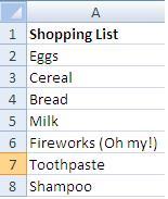
1. List all of the items that you wish to place in the drop-down menu, as shown below.

2. Highlight the list of items.
3. Click on the Insert tab in the Excel ribbon, and click Table to insert these items into a table.

4. A prompt will appear. If you have placed a title at the top of your list, check the ‘My table has headers’ box, or otherwise leave it unchecked. Click OK.

5. Highlight all of the items listed in the table, except for the title (unless you want to include it in the list).
6. Click into the name field, which should be currently displaying ‘Table1’, or something similar. Type in a name for the list. For this example, I’m going to call it ‘Shopping’.

The second stage is to turn our data into a dynamic list:

1. Select a new cell to place your drop-down menu in. For this example, I chose C1.
2. On the Excel ribbon, click on the Data tab and select Data Validation.

3. A prompt will appear. In the menu below Allow, select List. In the box below Source, type ‘=’ and then the name for your list (in this example ‘=Shopping’). Leave all other settings as they are and click OK.

The third stage is to test whether our list has worked.

1. Select the cell that you placed your menu in. An arrow should appear to the right of the cell.
2. Click on the arrow, and your items should display. If they don’t, then go back to the start of the second stage and repeat the steps again.

Finally, to add another item to the menu.

1. Click in the cell directly below your last list item, whichin this example is Shampoo.
2. Enter a new item. For this example, I’ll enter Balloons. Everybody here likes balloons, right?  Right.

Now go back to your menu and click on the arrow again. You should see the new item appear at the bottom.

Hooray! Even better is that it seems there is no limit to the amount of items you wish to include in your list. I added up to 530 items to the list and the menu held every single one of them.

And there you are – dynamic data validation lists!